Code
library(bayesrules)
library(tidyverse)
library(rstanarm)
library(tidybayes)
library(bayesplot)
library(broom.mixed)
library(patchwork)
library(janitor)

data(bikes)September 25, 2022
For the Normal regression model (9.6) with \(Y_i | \beta_0, \beta_1, \sigma \sim N(\mu_i, \sigma)\) where \(\mu_i = \beta_0 + \beta_1 X_i\), we utilized Normal priors for \(\beta_0\), \(\beta_1\) and an Exponential prior on \(\sigma\).
Identify the response variable (\(Y\)) and predictor variable (\(X\)) in each given relationship of interest.
In each situation below, suppose that the typical relationship between the given response variable \(Y\) and predictor \(X\) can be described by \(\beta_0 + \beta_1 X\). Interpret the meaning of \(\beta_0\) and \(\beta_1\) and indicate whether your prior understanding suggests that \(\beta_1\) is negative or positive.
Consider the Normal regression model (9.6). Explain in one or two sentences, in a way that one of your non-stats friends could understand, how \(\sigma\) is related to the strength of the relationship between a response variable \(Y\) and predictor \(X\).
Our data’s variability is measured by \(sigma\), which indicates that the lower the value, the less variable our data are. To give an example, if we know that our average data is 100 and that our variability is 10, we should anticipate that our data will vary by 10, demonstrating the tightness of our data and the strength of our predictor. The association between our predictor and outcome variables is weaker when our variability is 50, as opposed to low variability, which means that our data may vary by as much as 50.
A researcher wants to use a person’s age (in years) to predict their annual orange juice consumption (in gallons). Here you’ll build up a relevant Bayesian regression model, step by step.
Lorem
Repeat the above exercise for the following scenario. A researcher wishes to predict tomorrow’s high temperature by today’s high temperature.
Lorem
Mark each statement about posterior regression simulation as True or False.
Lorem
For each situation, specify the appropriate stan_glm() syntax for simulating the Normal regression model using 4 chains, each of length 10000. (You won’t actually run any code.)
age; \(Y\) = height; dataset name: bunnies.songs.dogs.Throughout this chapter, we explored how bike ridership fluctuates with temperature. But what about humidity? In the next exercises, you will explore the Normal regression model of rides (\(Y\)) by humidity (\(X\)) using the bikes dataset. Based on past bikeshare analyses, suppose we have the following prior understanding of this relationship:
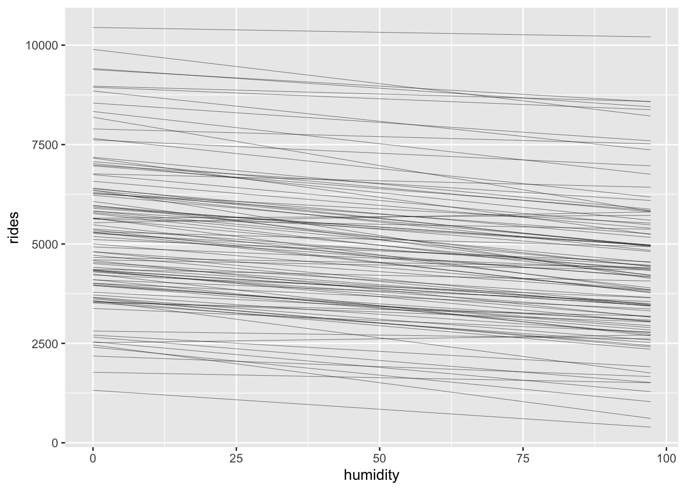
stan_glm() syntax that you would use to simulate the posterior, but include prior_PD = TRUE.$$ \[\begin{gather*} Y_i | \beta_0,\beta_1,\sigma∼N(\mu_i,\sigma^2) \; \;with \;\;\mu_i=\beta_0 + \beta_1 X_i \\ \beta_{0c} \sim N(5000, 2000) \\ \beta_1 \sim N(-10, 5) \\ \sigma \sim Exp(1/2000) \end{gather*}\] $$
bikes %>%
  add_epred_draws(bike_model_prior, ndraws = 100) %>%
  ggplot(aes(humidity, rides)) +
  geom_line(aes(y = .epred, group = .draw), size = 0.1)
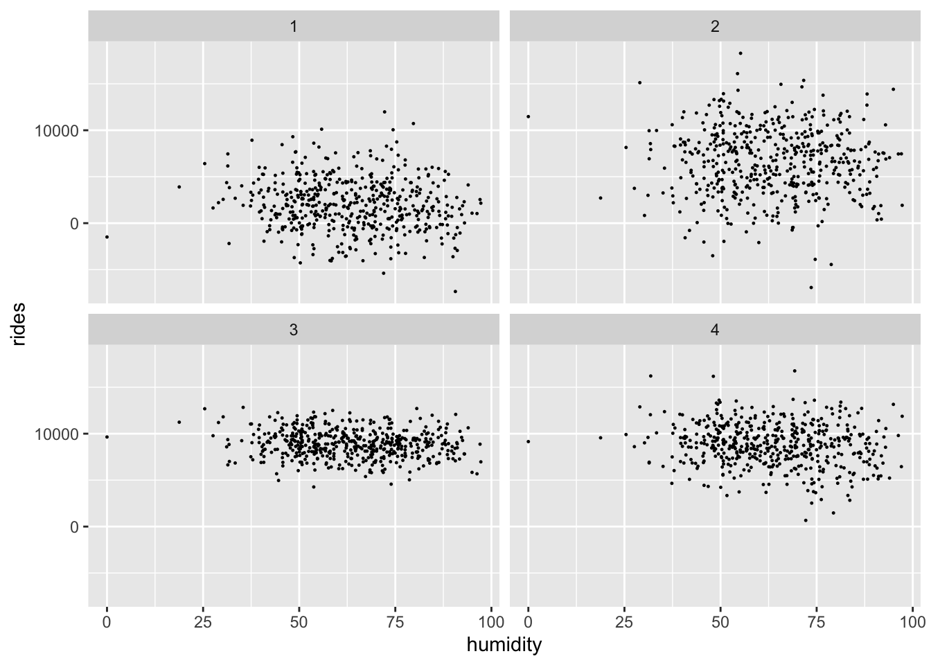
set.seed(12)

bikes %>%
  add_predicted_draws(bike_model_prior, ndraws = 4) %>%
  ggplot(aes(humidity, rides)) +
  geom_point(aes(y = .prediction, group = .draw), size = 0.2) +
  facet_wrap(~ .draw)
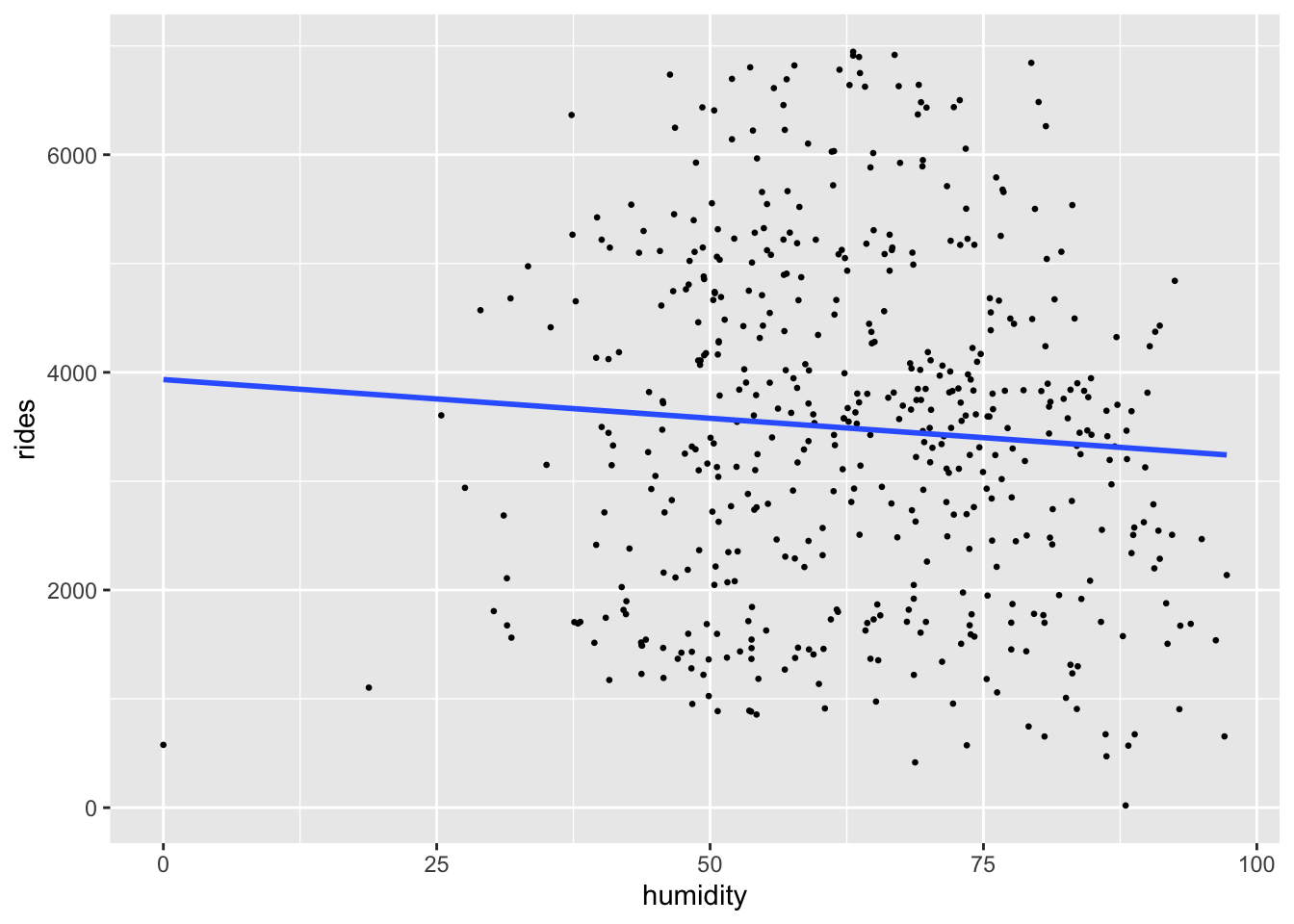
With the priors in place, let’s examine the data.
ggplot(bikes, aes(x = humidity, y = rides)) +
  geom_point(size = 0.5) +
  geom_smooth(method = "lm", se = FALSE)
We can now simulate our posterior model of the relationship between ridership and humidity, a balance between our prior understanding and the data.
stan_glm() to simulate the Normal regression posterior model. Do so with 5 chains run for 8000 iterations each. HINT: You can either do this from scratch or update() your prior simulation from Exercise 9.9 using prior_PD = FALSE.(Intercept) humidity sigma
1.01665 1.03015 1.04410 (Intercept) humidity sigma
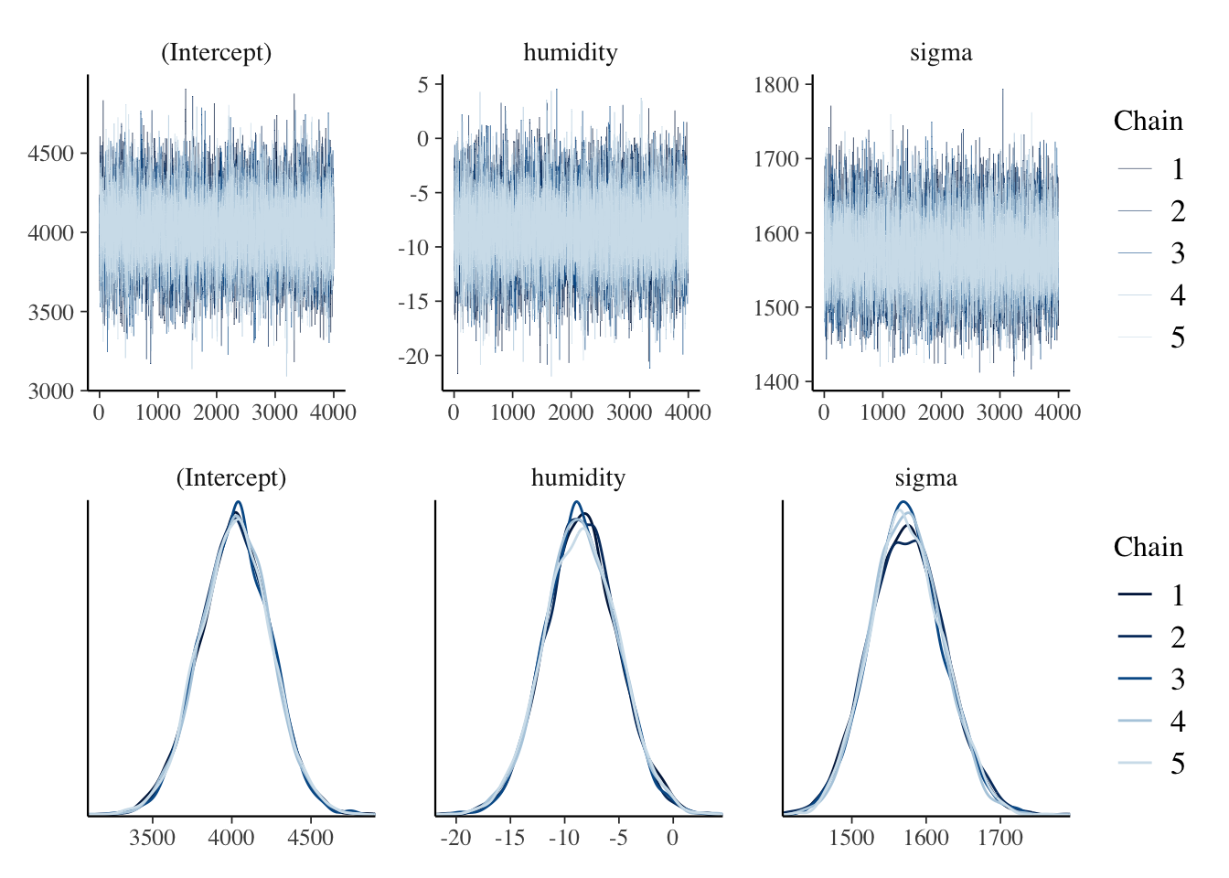
0.9999646 0.9999129 0.9998725 # Trace plots of parallel chains
trace_plot <- mcmc_trace(bike_model, size = 0.1)
# Density plots of parallel chains
density_plot <- mcmc_dens_overlay(bike_model)
trace_plot / density_plot
Finally, let’s dig deeper into our posterior understanding of the relationship between ridership and humidity.
tidy() summary of your posterior model, including 95% credible intervals.humidity coefficient, \(\beta_1\).# Posterior summary statistics
tidy(bike_model, effects = c("fixed", "aux"),
conf.int = TRUE, conf.level = 0.95)# A tibble: 4 × 5
term estimate std.error conf.low conf.high
<chr> <dbl> <dbl> <dbl> <dbl>
1 (Intercept) 4023. 225. 3580. 4457.
2 humidity -8.50 3.36 -15.0 -1.78
3 sigma 1573. 49.3 1480. 1672.
4 mean_PPD 3483. 99.7 3291. 3678. Based on the table above, we estimated that the \(\sigma\) has a posterior median of 1573, with 95% credible interval of [1481, 1674]. That means we expect the ridership on a given day could be as high or as low as 1573 riders from the average ridership on the same day and the same humidity.
The 95% credible interval indicates that the humidity coefficient (\(\beta_1\)) could be anywhere between -15 to -1.8.
Yes, we have an ample evidence that there’s negative association between ridership and humidity. First, based on the visual inspection from the posterior we plotted above, we saw negative association between ridership and humidity. Had no association or positive association, the figure above would showed a flat or positive slope. Second, the posterior summary statistics for the humidity showed that the credible interval had no overlap with zero. Lastly, the quick tabulation from posterior probability showed that there’s almost certainly positive association between ridership and humidity.
Tomorrow is supposed to be 90% humidity in Washington, D.C. What levels of ridership should we expect?
posterior_predict() shortcut function, simulate two posterior models:posterior_predict() to confirm the results from your posterior predictive model of tomorrow’s ridership.predict_90 <- bike_model_df %>%
mutate(mu = `(Intercept)` + humidity * 90,
y_new = rnorm(20000, mean = mu, sd = sigma))
predict_90 %>%
summarize(
median_mu = quantile(mu, 0.5),
lower_mu = quantile(mu, 0.025),
upper_mu = quantile(mu, 0.975),
median_new = quantile(y_new, 0.5),
lower_new = quantile(y_new, 0.025),
upper_new = quantile(y_new, 0.975)
) median_mu lower_mu upper_mu median_new lower_new upper_new
1 3259.577 3034.744 3483.41 3252.493 184.4085 6358.909