BDA GSU 2021 Project: Roaches

Introduction

In this mini-project, we would like to estimate the efficacy of integrated pest management on reducing cockroach levels in urban apartments. This problem has been previously illustrated in Chapter 15 of Gelman, Hill, and Vehtari’s Regression and Other Stories (2020). In the experiment, the study is performed to 160 treatment apartments and 104 control apartments with the outcome \(y_i\) in the \(i\) apartment was the number of cockroaches caught in the trap. Since the number of days for which the traps were different on each apartment, we need to take into account the exposure2 variable. The data itself were obtained from the rstanarm library. The variables from roaches dataset, namely the number of cockroaches roach1, treatment indicator treatment, and the variable whether the apartment was restricted to the elderly resident senior, were included as predictors into the model. Since we were dealing with count data and the outcome variable did not have a natural limit, then it is standard to use the Poisson and Negative Binomial model. Later, we will explore another model, the Zero Inflated Negative Binomial, because our data have more zero outcomes than predicted by the model.

Our analysis would be different from the existing analysis because we would incorporate several prior choices to analyze the sensitivity of our model. Furthermore, we would provide the convergence diagnostics for each model to assess if our model reached stationary and well-mixed. The rest of the bayesian workflow, such as prior predictive check, posterior predictive check, and model comparison will be included throughout the analysis. Before we jump into the modeling realm, we need to understand the data better by generating summary statistics, and visualizing the variable distribution and its relation to other variables.

Data Exploration

library(tidyverse)
library(here)
library(bayesplot)
library(loo)
library(knitr)
library(janitor)

library(brms)
library(rstanarm)
library(rstan)
rstan_options(auto_write = TRUE)
options(mc.cores = parallel::detectCores())
rstan_options(javascript=FALSE)

theme_set(theme_minimal())

# For reproducibility
SEED <- 12

data(roaches) 
roaches %>% 
  select(exposure2, roach1, y) %>% 
  pivot_longer(everything()) %>% 
  ggplot(aes(value)) + 
  geom_histogram(aes(y = ..ncount..)) + 
  geom_density(aes(y = ..scaled..)) + 
  facet_wrap(~name, scales = "free")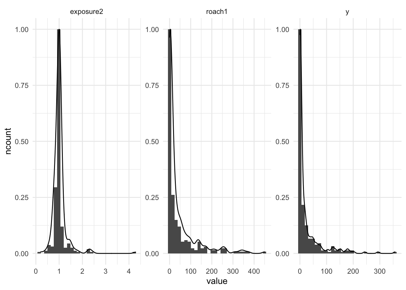

Based on the histogram above, the roach1 and y variables have a lot zero values, which right skewed the distribution. We could scale down the roach1 by divided with 100.

roaches <- roaches %>% 
  mutate(roach100 = roach1 / 100, 
         y_log = log(y + 1))

roaches %>% 
  select(senior, treatment) %>% 
  pivot_longer(everything()) %>% 
  ggplot(aes(value)) + 
  geom_bar() + 
  coord_flip() + 
  facet_wrap(~name, scales = "free")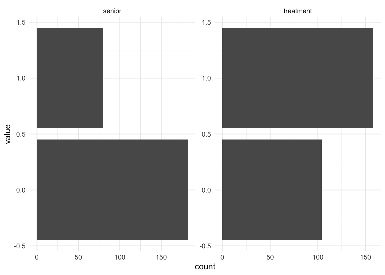

Moreover, the senior variable has an imbalance ratio, where the senior-only apartment was significantly lower than its counterpart, while the apartment with treatment are higher than control, as seen in the above figures.

roaches %>% 
  group_by(senior) %>% 
  summarise(roach1 = sum(roach1) / n()) %>% 
  ungroup()

# A tibble: 2 × 2
  senior roach1
   <int>  <dbl>
1      0   48.7
2      1   27.4

Before the treatment, the senior apartment cockroaches level was on average was lower (27.3%) compared to the non senior apartment (48.7%).

roaches %>% 
  group_by(treatment) %>% 
  summarise(y = sum(y), 
            roach1 = sum(roach1)) %>% 
  ungroup() %>% 
  mutate(percentage = round((roach1 - y) / roach1, 2))

# A tibble: 2 × 4
  treatment     y roach1 percentage
      <int> <int>  <dbl>      <dbl>
1         0  3607  4219.       0.15
2         1  3113  6835.       0.54

Based on the summary above, the reduction of roaches after the treatment was relatively higher, compared to the control experiment. The pest management might be effective in reducing the cockroach levels.

Model

Since our model is in the log scale, the regression coefficients are typically in the range -1 and 1. Hence, we could assign the prior to Normal distribution with \(\mu = 0\) and \(\sigma = 1\). 95% of the distribution covered the value from -2 to 2. We will fit the model using all the predictors we have in the data.

Poisson Model

First, we fit the Poisson model:

poisson_model <- here("stan_files", "project_poisson.stan")
roaches_data <- list(N = nrow(roaches), treatment = roaches$treatment, 
                     senior = roaches$senior, roaches100 = roaches$roach100, 
                     y = roaches$y, exposure2 = roaches$exposure2,
                     prior_mu = 0, prior_sd = 1)
poisson_fit <- stan(file = poisson_model, data = roaches_data, seed = SEED, 
                    refresh = 0)
print(poisson_fit, pars = c("treatment_coef", "senior_coef", "roaches100_coef", 
                            "Intercept"))

Inference for Stan model: project_poisson.
4 chains, each with iter=2000; warmup=1000; thin=1; 
post-warmup draws per chain=1000, total post-warmup draws=4000.

                 mean se_mean   sd  2.5%   25%   50%   75% 97.5% n_eff Rhat
treatment_coef  -0.52       0 0.02 -0.56 -0.53 -0.52 -0.50 -0.47  2345    1
senior_coef     -0.38       0 0.03 -0.44 -0.40 -0.38 -0.36 -0.31  2884    1
roaches100_coef  0.70       0 0.01  0.68  0.69  0.70  0.70  0.72  2530    1
Intercept        3.09       0 0.02  3.05  3.07  3.09  3.10  3.13  1987    1

Samples were drawn using NUTS(diag_e) at Fri Sep  9 20:44:26 2022.
For each parameter, n_eff is a crude measure of effective sample size,
and Rhat is the potential scale reduction factor on split chains (at 
convergence, Rhat=1).

mcmc_trace(poisson_fit, regex_pars = "coef|Intercept")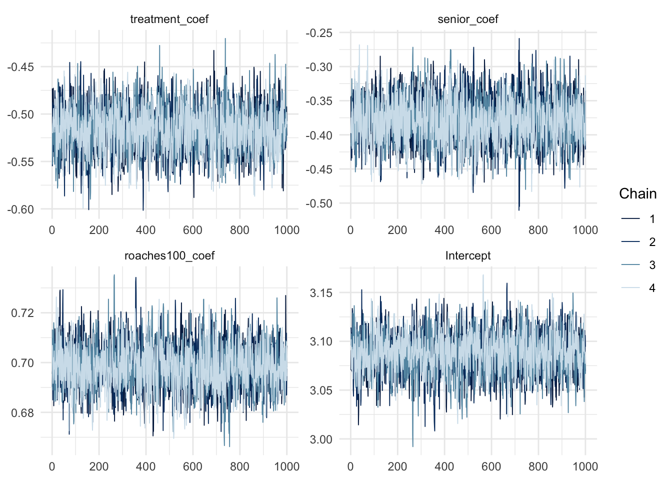

As shown in the table above, The \(\widehat{R}\) values is close to one, meaning our chains probably converged and the estimates are deemed reliable. Furthermore, The chains have mixed well, have reached stationary and traced out a common distribution. So, visually speaking, the chains have reached convergence.

To check if the model fit the data well, we simulated the replicated yrep given that our model was true and compared with the actual y.

poisson_yrep <- as.data.frame(poisson_fit, pars = "yrep") %>% 
  slice(1:200) %>% 
  as.matrix()

ppc_dens_overlay(roaches$y_log, log(poisson_yrep + 1))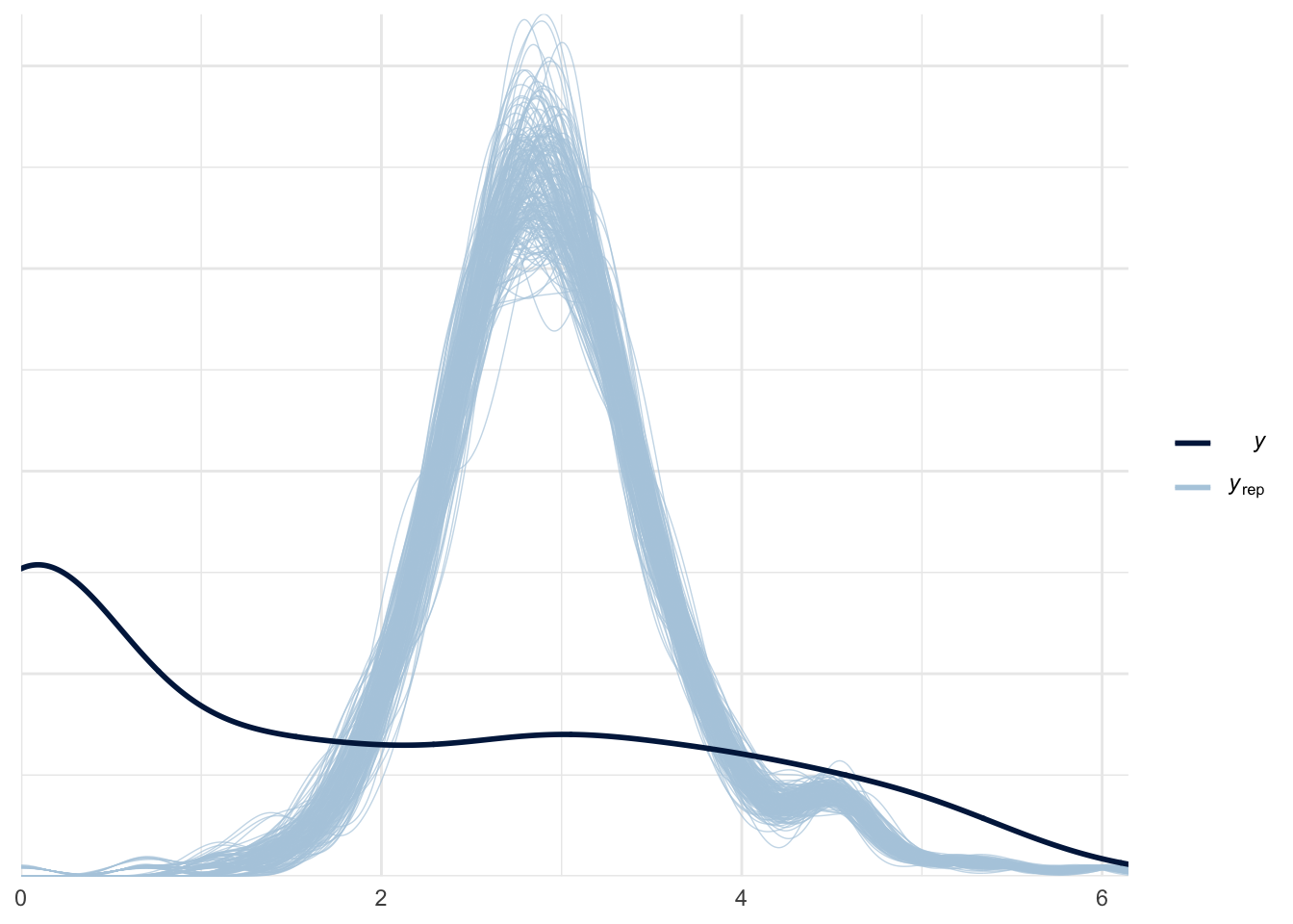

Our model seems to perform poorly. The reason might be that the actual data has a lot of zeros, and our model failed to accurately account the large proportion of zeros in the data. Let’s compute the proportion of zeros from our model against the actual data:

ppc_stat(y=roaches$y, yrep=poisson_yrep, stat=function(y) mean(y==0))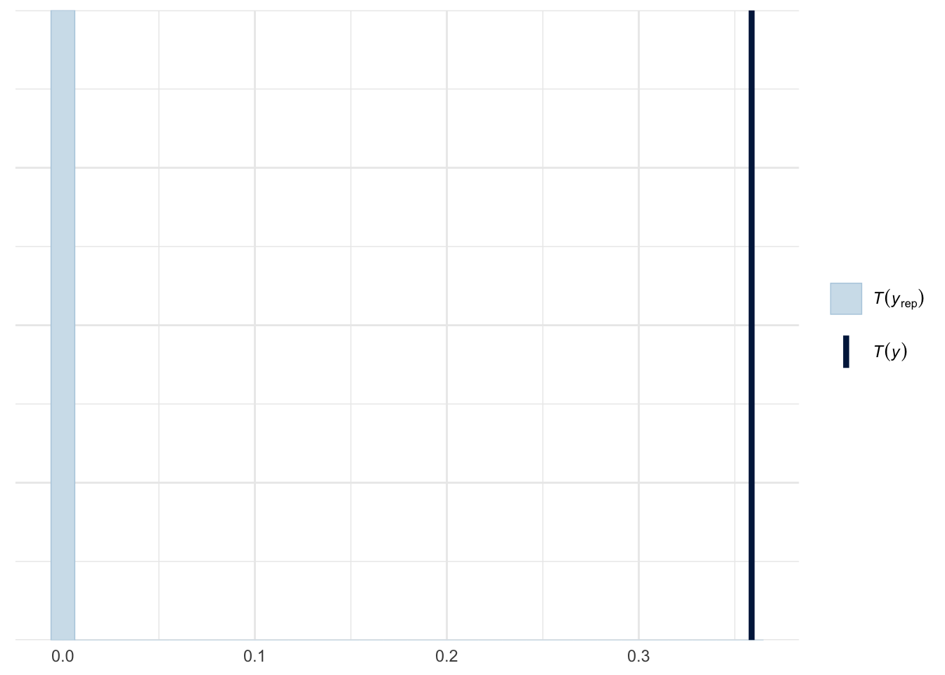

As we expected, the model failed to capture the high percentage of zeros from the actual data. More than 30% of the observed data are zeros as shown in dark blue line, while our model predict less than 1% zeros as shown in light blue.

Negative Binomial Model

In order to alleviate the problem with our model, we will try to fit using the negative binomial which is used for overdispersed or zero-inflated count data.

negbinom_model <- here("stan_files", "project_negbinom.stan")
roaches_data <- list(N = nrow(roaches), treatment = roaches$treatment, 
                     senior = roaches$senior, roaches100 = roaches$roach100, 
                     y = roaches$y, exposure2 = roaches$exposure2, 
                     prior_mu = 0, prior_sd = 1)
negbinom_fit <- stan(file = negbinom_model, data = roaches_data, seed = SEED, 
                    refresh = 0)
print(negbinom_fit, pars = c("treatment_coef", "senior_coef", "roaches100_coef", 
                            "Intercept", "phi"))

Inference for Stan model: project_negbinom.
4 chains, each with iter=2000; warmup=1000; thin=1; 
post-warmup draws per chain=1000, total post-warmup draws=4000.

                 mean se_mean   sd  2.5%   25%   50%   75% 97.5% n_eff Rhat
treatment_coef  -0.65       0 0.23 -1.11 -0.80 -0.65 -0.50 -0.21  2949    1
senior_coef     -0.26       0 0.25 -0.74 -0.43 -0.27 -0.09  0.24  2852    1
roaches100_coef  1.31       0 0.24  0.86  1.14  1.30  1.47  1.80  3161    1
Intercept        2.72       0 0.21  2.32  2.57  2.71  2.86  3.15  2172    1
phi              0.27       0 0.03  0.22  0.25  0.27  0.29  0.33  3307    1

Samples were drawn using NUTS(diag_e) at Fri Sep  9 20:45:03 2022.
For each parameter, n_eff is a crude measure of effective sample size,
and Rhat is the potential scale reduction factor on split chains (at 
convergence, Rhat=1).

mcmc_trace(negbinom_fit, regex_pars = "coef|Intercept|phi")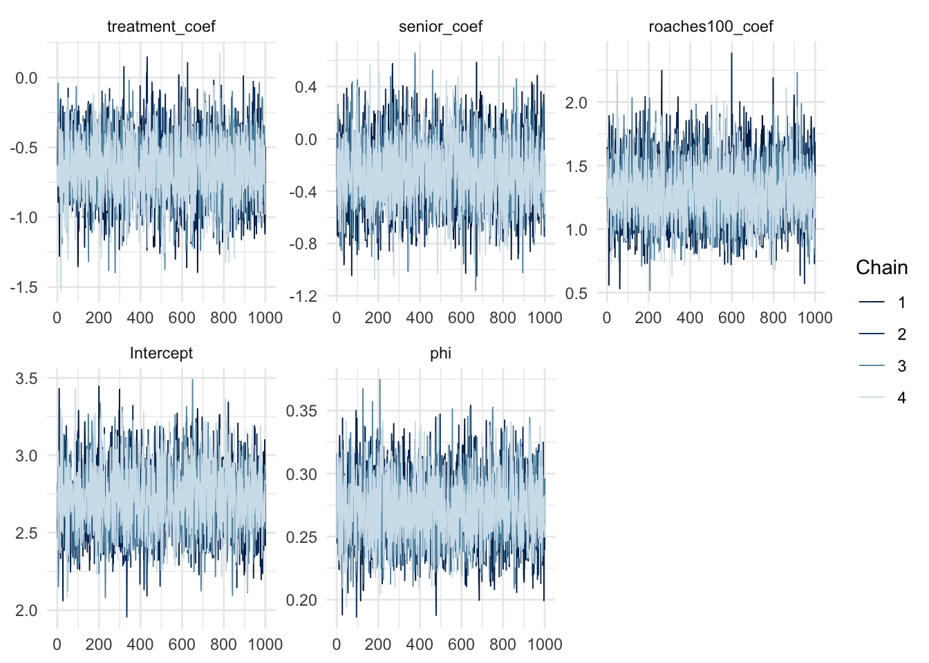

The model also fit without any problem, as seen from the \(\widehat{R}\) values and the chains trace plot. Similarly, we would also check the posterior predictive distribution and the zeros proportion test:

negbinom_yrep <- as.data.frame(negbinom_fit) %>% 
  select(contains("yrep")) %>%
  slice(1:200) %>% 
  as.matrix()

ppc_dens_overlay(roaches$y_log, log(negbinom_yrep + 1))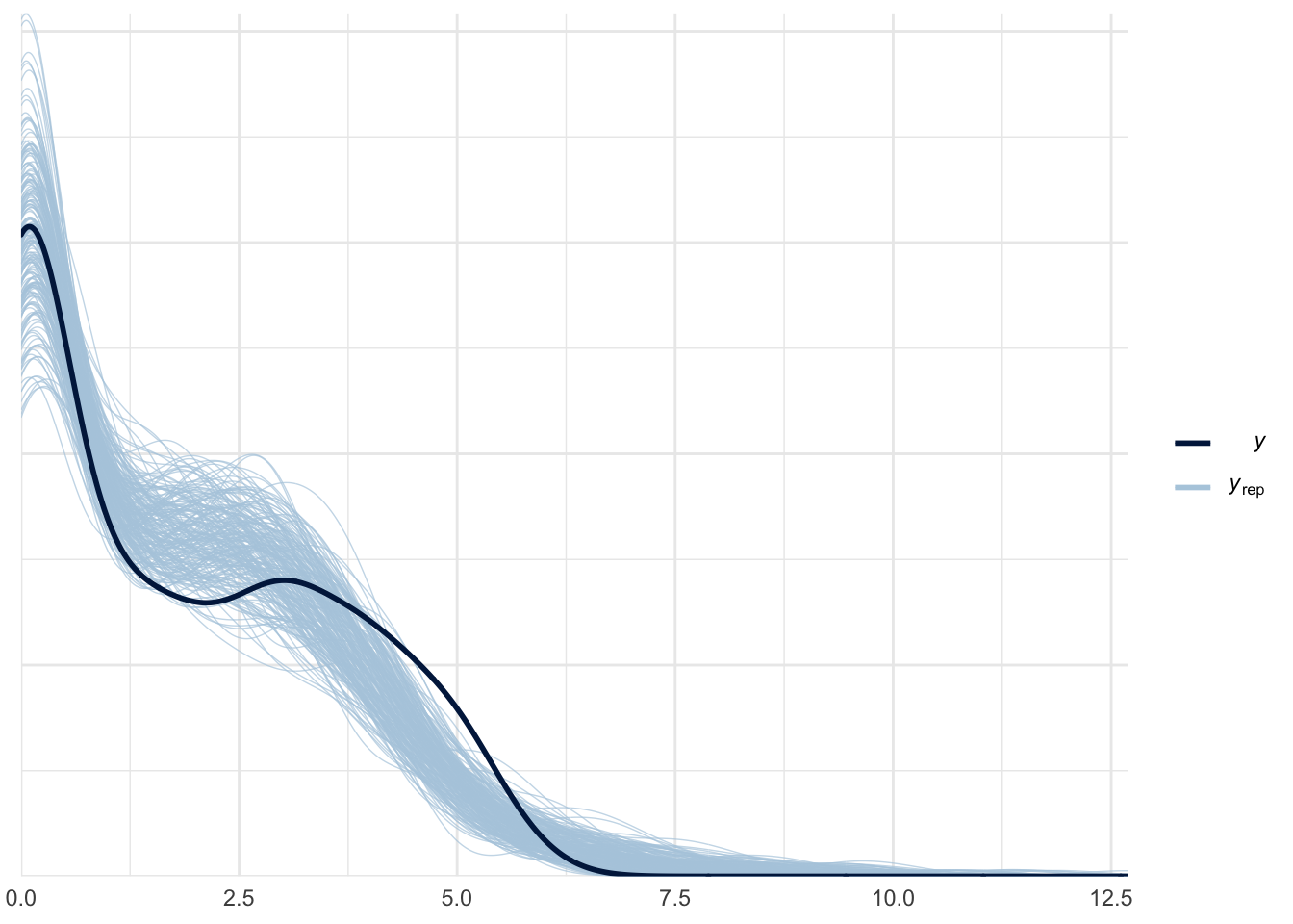

ppc_stat(y=roaches$y, yrep=negbinom_yrep, stat=function(y) mean(y==0))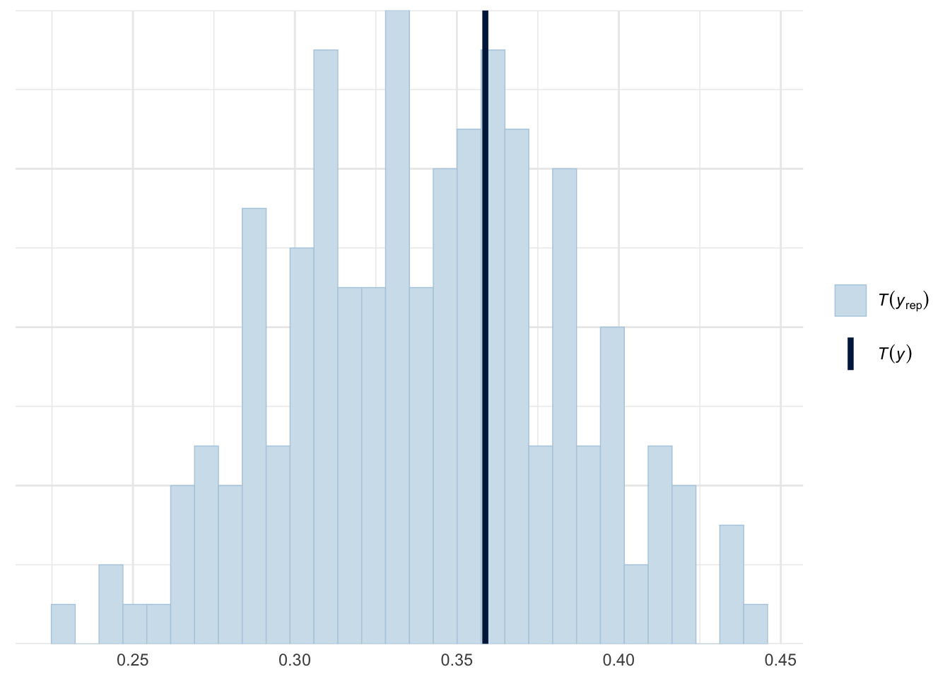

The negative binomial model is clearly better than the poisson model. The posterior predictive distribution and the zeros proportion from the actual data fell really well in our simulated dataset. To compare the fit of the two models, we can use Pareto-smoothed importance sampling leave-one-out cross-validation as model checking tool.

negbinom_loo <- loo(negbinom_fit)

Warning: Some Pareto k diagnostic values are slightly high. See help('pareto-k-diagnostic') for details.

poisson_loo <- loo(poisson_fit)

Warning: Some Pareto k diagnostic values are too high. See help('pareto-k-diagnostic') for details.

loo_compare(poisson_loo, negbinom_loo)

       elpd_diff se_diff
model2     0.0       0.0
model1 -5353.0     709.5

Even though there is some influential observation due to model misspecification, the comparison indicates that negative binomial is better than Poisson.

Zero Inflated Negative Binomial Model

As the zeros observation are quite high, we might as well try the Zero Inflated Negative Binomial model. The following code run the said model:

zinb_model <- here( "stan_files", "project_zinb.stan")
roaches_data <- list(N = nrow(roaches), treatment = roaches$treatment, 
                     senior = roaches$senior, roaches100 = roaches$roach100, 
                     y = roaches$y, exposure2 = roaches$exposure2, 
                     prior_mu = 0, prior_sd = 1)
zinb_fit <- stan(file = zinb_model, data = roaches_data, seed = SEED,
                    refresh = 0)
variables <- c("treatment_coef", "senior_coef", "roaches100_coef", 
               "Intercept", "phi", "treatment_zi_coef", "senior_zi_coef",
               "roaches100_zi_coef", "Intercept_zi")
print(zinb_fit, pars = variables)

Inference for Stan model: project_zinb.
4 chains, each with iter=2000; warmup=1000; thin=1; 
post-warmup draws per chain=1000, total post-warmup draws=4000.

                    mean se_mean   sd  2.5%   25%   50%   75% 97.5% n_eff Rhat
treatment_coef     -0.48    0.00 0.21 -0.89 -0.62 -0.48 -0.34 -0.07  4735    1
senior_coef        -0.02    0.00 0.25 -0.51 -0.18 -0.02  0.15  0.47  4602    1
roaches100_coef     0.92    0.00 0.17  0.62  0.81  0.91  1.02  1.26  4228    1
Intercept           3.05    0.00 0.19  2.69  2.92  3.04  3.17  3.43  3534    1
phi                 0.49    0.00 0.06  0.37  0.45  0.49  0.53  0.62  4285    1
treatment_zi_coef   0.62    0.01 0.39 -0.13  0.36  0.62  0.88  1.38  4073    1
senior_zi_coef      0.98    0.01 0.37  0.26  0.74  0.98  1.22  1.73  4527    1
roaches100_zi_coef -3.03    0.01 0.70 -4.46 -3.49 -3.00 -2.53 -1.72  4953    1
Intercept_zi       -1.21    0.01 0.37 -1.96 -1.44 -1.19 -0.95 -0.55  3294    1

Samples were drawn using NUTS(diag_e) at Fri Sep  9 20:45:51 2022.
For each parameter, n_eff is a crude measure of effective sample size,
and Rhat is the potential scale reduction factor on split chains (at 
convergence, Rhat=1).

mcmc_trace(zinb_fit, regex_pars = "coef|Intercept|phi")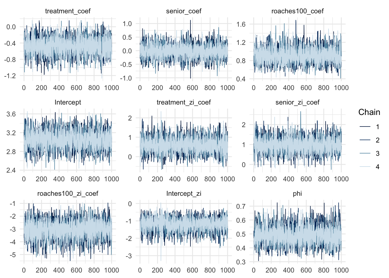

The \(\widehat{R}\) values and the chains trace plot showed the model fit without any problem. Let’s check the posterior predictive distribution and the zeros proportion test:

zinb_yrep <- as.data.frame(zinb_fit, pars = "yrep") %>% 
  slice(1:200) %>% 
  as.matrix()

ppc_dens_overlay(roaches$y_log, log(zinb_yrep + 1))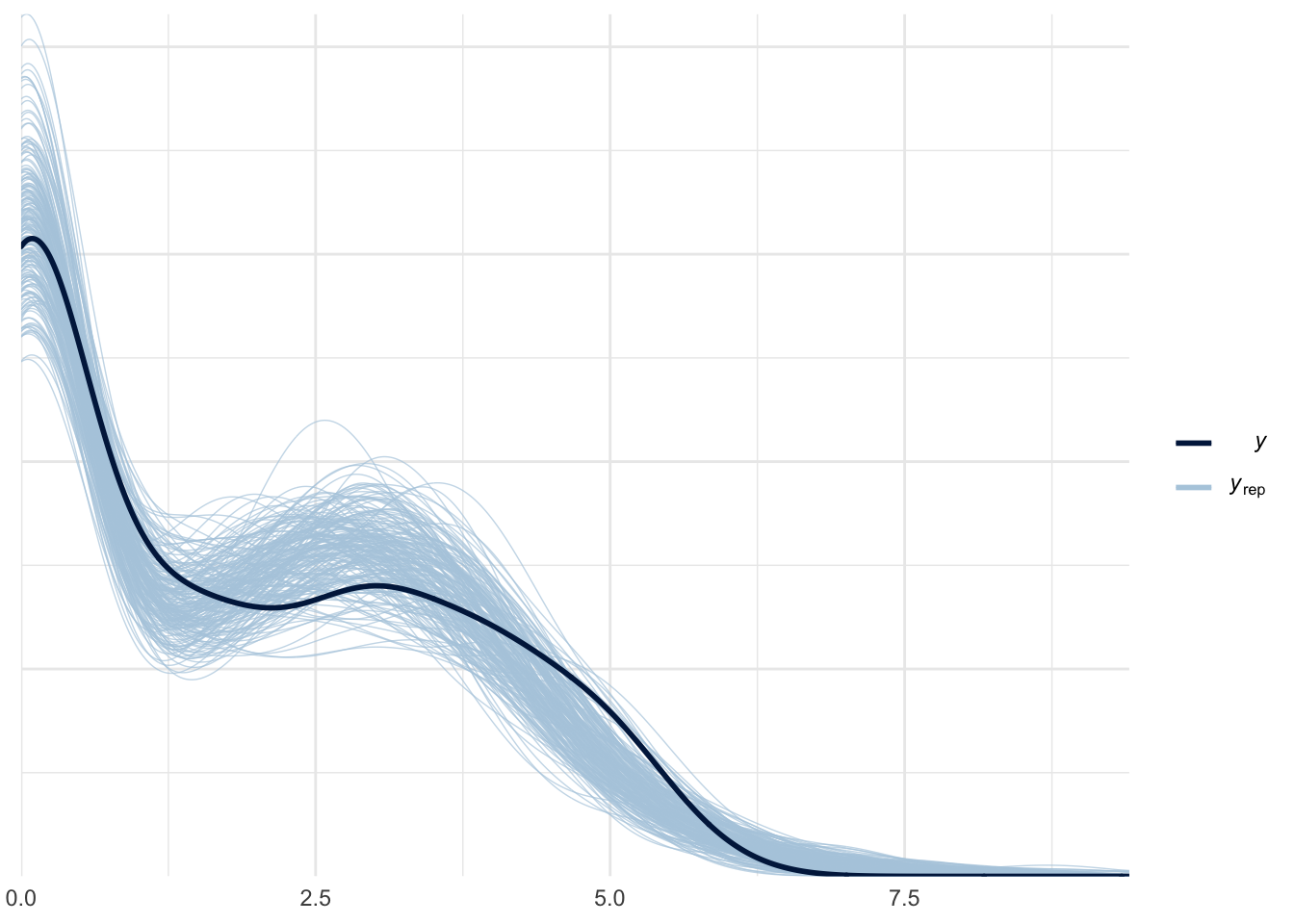

ppc_stat(y=roaches$y, yrep=zinb_yrep, stat=function(y) mean(y==0))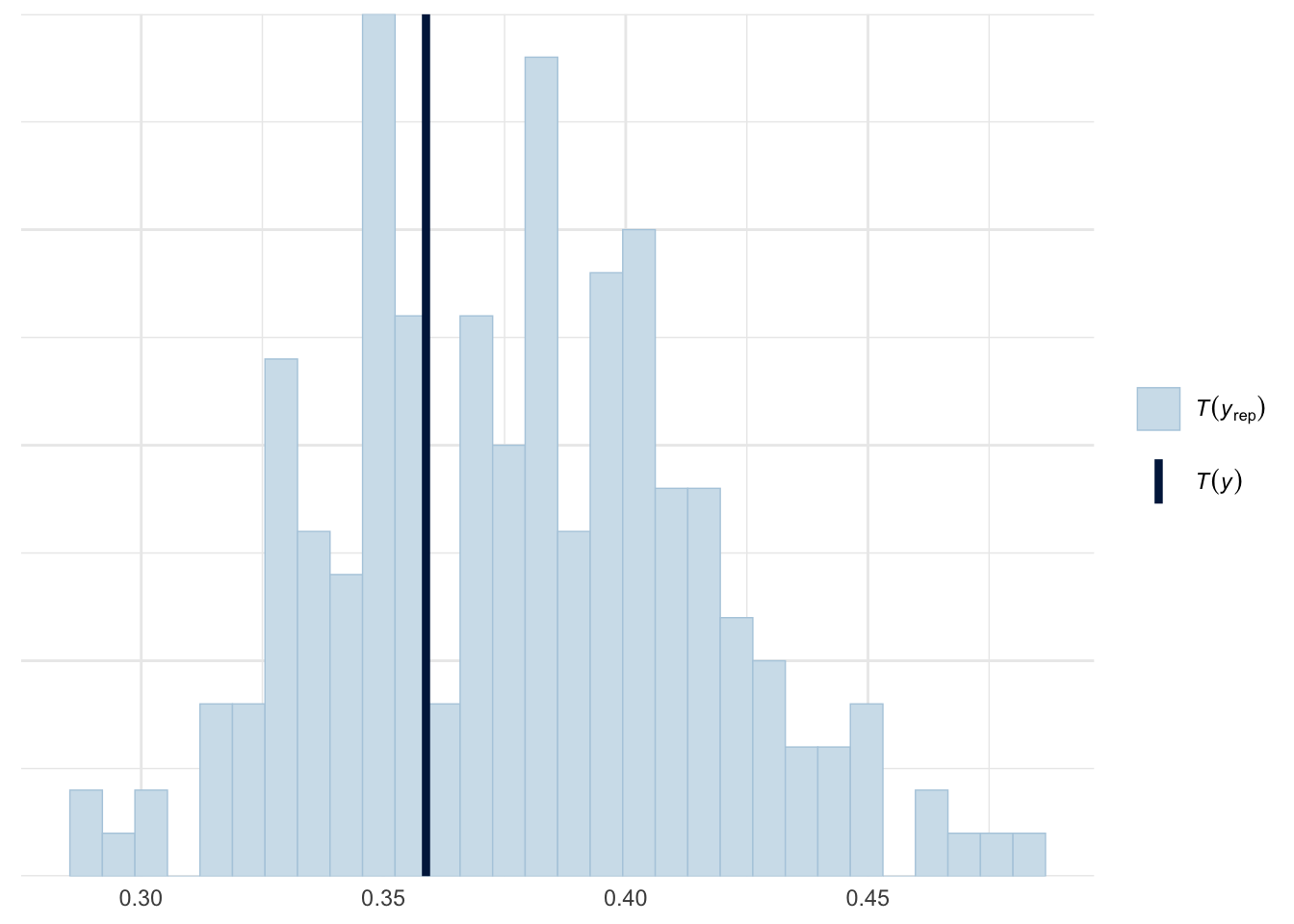

zinb_loo <- loo(zinb_fit)

Warning: Some Pareto k diagnostic values are too high. See help('pareto-k-diagnostic') for details.

loo_compare(negbinom_loo, zinb_loo)

       elpd_diff se_diff
model2   0.0       0.0  
model1 -17.4       5.6  

the posterior predictive distribution, the zeros proportion test and the LOO showed a promising result that the Zero Inflated Negative Binomial model fit the model really well. To check how our model changed by using weakly informative prior, we will set the \(\sigma = 10\).

zinb_model <- here("stan_files", "project_zinb.stan")
roaches_data <- list(N = nrow(roaches), treatment = roaches$treatment, 
                     senior = roaches$senior, roaches100 = roaches$roach100, 
                     y = roaches$y, exposure2 = roaches$exposure2, 
                     prior_mu = 0, prior_sd = 10)
zinb_fit_2 <- stan(file = zinb_model, data = roaches_data, seed = SEED,
                    refresh = 0)
variables <- c("treatment_coef", "senior_coef", "roaches100_coef", 
               "Intercept", "phi", "treatment_zi_coef", "senior_zi_coef",
               "roaches100_zi_coef", "Intercept_zi")

mcmc_areas(zinb_fit, regex_pars = "coef|Intercept|phi")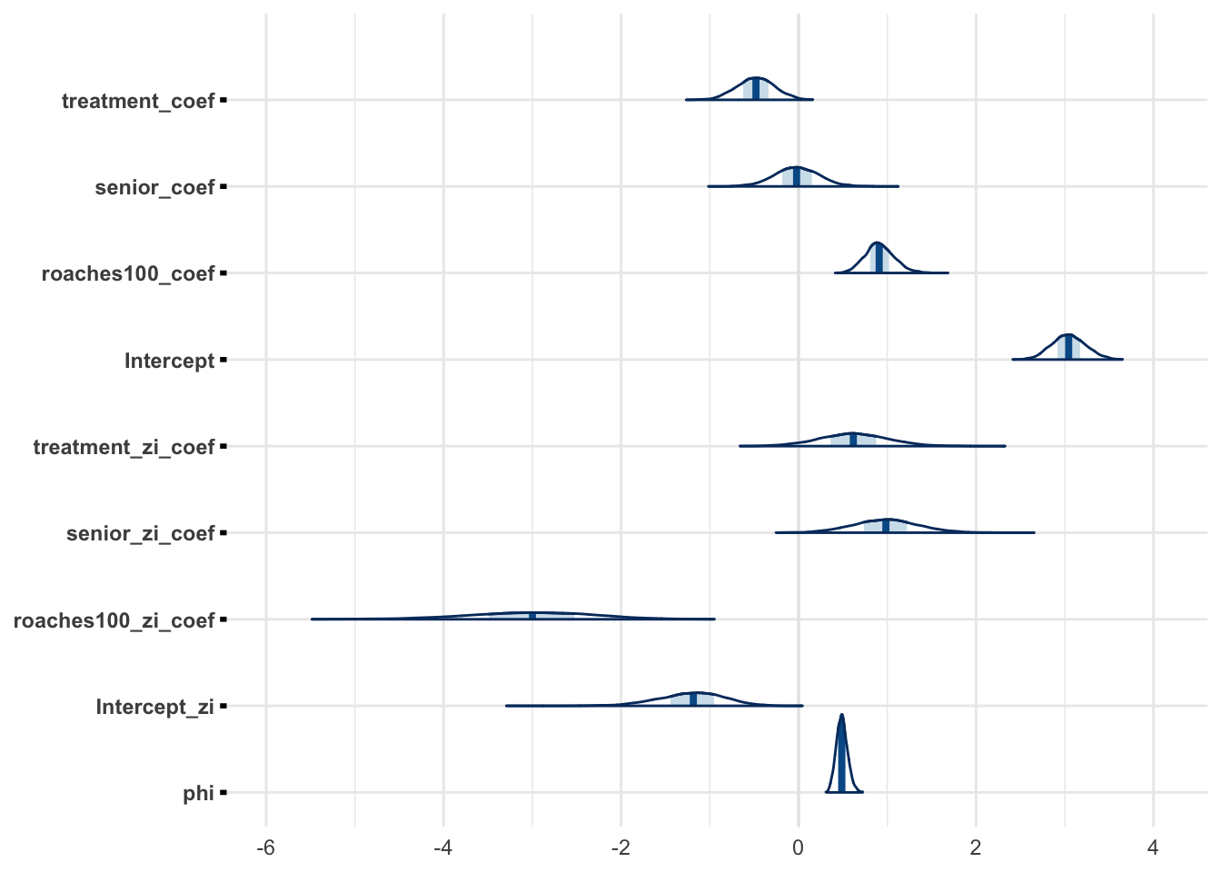

mcmc_areas(zinb_fit_2, regex_pars = "coef|Intercept|phi")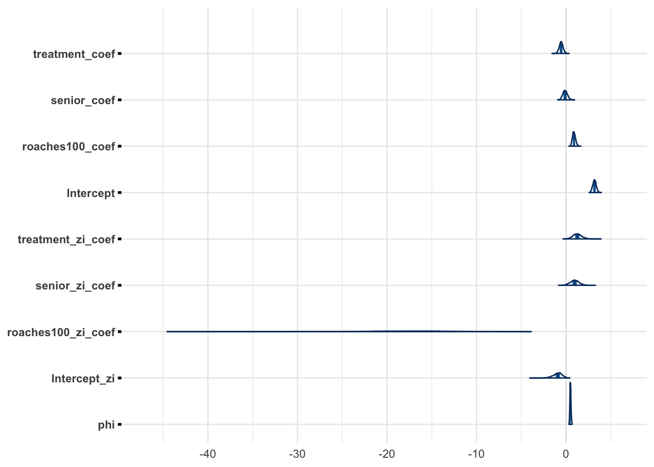

The marginals for weakly informative prior is similar to marginals with the informative prior.

Conclusion

We have explore various models, namely Poisson, Negative Binomial, and Zero Inflated Negative Binomial, to find the best model that fit the observed data. While the Poisson has some potential problem, the Negative Binomial managed to alleviate the problem, and even better the Zero Inflated Negative Binomial captured the observed data well.

Apendix

Poisson Stan Model

data {
  int<lower=0> N;                     // Number of observations
  vector[N] treatment;                // Treatment column
  vector[N] senior;                   // Senior column
  vector[N] roaches100;               // Pre-treatment roaches column
  int<lower=0> y[N];                  // Roaches column
  vector[N] exposure2;                // Exposure column
  real prior_mu;                      // prior mu for all predictors
  real prior_sd;                      // prior sd for all predictors
}

parameters {
  real treatment_coef;    // Treatment column
  real senior_coef;       // Senior column
  real roaches100_coef;   // Pre-treatment roaches column
  real Intercept;
}

transformed parameters {
  vector[N] mu;
  mu = Intercept + treatment_coef * treatment + senior_coef * senior + 
       roaches100_coef * roaches100 + log(exposure2);
}

model {
  // Priors
  treatment_coef ~ normal(prior_mu, prior_sd);
  senior_coef ~ normal(prior_mu, prior_sd);
  roaches100_coef ~ normal(prior_mu, prior_sd);
  Intercept ~ normal(prior_mu, prior_sd);
  
  // Likelihood
  y ~ poisson_log(mu);
}

generated quantities {
  int yrep[N] = poisson_log_rng(mu);
  real log_lik[N];
  for (i in 1:N) {
    log_lik[i] = poisson_log_lpmf(y[i] | mu[i]);
    }
}

Negative Binomial Stan Model

data {
  int<lower=0> N;                     // Number of observations
  vector[N] treatment;                // Treatment column
  vector[N] senior;                   // Senior column
  vector[N] roaches100;               // Pre-treatment roaches column
  int<lower=0> y[N];                  // Roaches column
  vector[N] exposure2;                // Exposure column
  real prior_mu;                      // prior mu for all predictors
  real prior_sd;                      // prior sd for all predictors
}

parameters {
  real treatment_coef;    // Treatment column
  real senior_coef;       // Senior column
  real roaches100_coef;   // Pre-treatment roaches column
  real Intercept;
  real phi;
}

transformed parameters {
  vector[N] mu;
  mu = Intercept + treatment_coef * treatment + senior_coef * senior + 
       roaches100_coef * roaches100 + log(exposure2);
}

model {
  // Priors
  treatment_coef ~ normal(prior_mu, prior_sd);
  senior_coef ~ normal(prior_mu, prior_sd);
  roaches100_coef ~ normal(prior_mu, prior_sd);
  Intercept ~ normal(prior_mu, prior_sd);
  phi ~ exponential(1);
  
  // Likelihood
  y ~ neg_binomial_2_log(mu, phi);
}

generated quantities {
  int yrep[N] = neg_binomial_2_log_rng(mu, phi);
  vector[N] log_lik;
  for (i in 1:N)
    log_lik[i] = neg_binomial_2_log_lpmf(y[i] | mu[i], phi);
}

Zero Inflated Negative Binomial Stan Model

data {
  int<lower=0> N;                     // Number of observations
  vector[N] treatment;                // Treatment column
  vector[N] senior;                   // Senior column
  vector[N] roaches100;               // Pre-treatment roaches column
  int<lower=0> y[N];                  // Roaches column
  vector[N] exposure2;                // Exposure column
  real prior_mu;                      // prior mu for all predictors
  real prior_sd;                      // prior sd for all predictors
}

parameters {
  real treatment_coef;    // Treatment column
  real senior_coef;       // Senior column
  real roaches100_coef;   // Pre-treatment roaches column
  real Intercept;
  real treatment_zi_coef;    // Treatment column
  real senior_zi_coef;       // Senior column
  real roaches100_zi_coef;   // Pre-treatment roaches column
  real Intercept_zi;
  real phi;
}

transformed parameters {
  vector[N] mu = Intercept + treatment_coef * treatment + senior_coef * senior + 
       roaches100_coef * roaches100 + log(exposure2);
  vector[N] zi = Intercept_zi + treatment_zi_coef * treatment + senior_zi_coef * senior + 
       roaches100_zi_coef * roaches100 + log(exposure2);
}

model {
  // Priors
  treatment_coef ~ normal(prior_mu, prior_sd);
  senior_coef ~ normal(prior_mu, prior_sd);
  roaches100_coef ~ normal(prior_mu, prior_sd);
  Intercept ~ normal(prior_mu, prior_sd);
  treatment_zi_coef ~ normal(prior_mu, prior_sd);
  senior_zi_coef ~ normal(prior_mu, prior_sd);
  roaches100_zi_coef ~ normal(prior_mu, prior_sd);
  Intercept_zi ~ normal(prior_mu, prior_sd);
  phi ~ exponential(1);

  for (i in 1:N) {
    if (y[i] == 0) { 
      target += log_sum_exp(bernoulli_logit_lpmf(1 | zi[i]), 
                         bernoulli_logit_lpmf(0 | zi[i]) + 
                         neg_binomial_2_log_lpmf(0 | mu[i], phi));
    } else { 
      target += bernoulli_logit_lpmf(0 | zi[i]) +  
             neg_binomial_2_log_lpmf(y[i] | mu[i], phi); 
    } 
  }
}

generated quantities { 
  int yrep[N];
  vector[N] log_lik;
  
  for (i in 1:N) {
  
     if (bernoulli_logit_rng(zi[i]) == 1) {
         yrep[i] = 0;
     } else {
             yrep[i] = neg_binomial_2_log_rng(mu[i], phi);
     }
  
  
     if (y[i] == 0) {
         /* Zero case */
         log_lik[i] = log_sum_exp(bernoulli_logit_lpmf(1 | zi[i]),
                                  bernoulli_logit_lpmf(0 | zi[i]) +
                                  neg_binomial_2_log_lpmf(0 | mu[i], phi));
     } else {
         log_lik[i] = bernoulli_logit_lpmf(0 | zi[i]) +
             neg_binomial_2_log_lpmf(y[i] | mu[i], phi);
     }
  
  }
}