Bayesian Review

Introduction

Imagine you are buying a new book on an e-commerce platform, and there are several sellers who offer that book. Because of past negative experiences with online purchases, you look at the sellers’ review ratings as your guide to choose where to buy.

• Seller #1: 100% positive reviews from 10 reviewers.
• Seller #2: 97% positive reviews from 100 reviewers.
• Seller #3: 94.3% positive reviews from 1000 reviewers.

Given this situation, which seller would you choose?

Experiment

We are tempted to choose seller #1, as those perfect 100% positive reviews would definitely give you reassurance to buy from them. But, let’s put this into another perspective. Let’s say that each seller has their true positive rate, which means there is a constant that defines how well the seller runs their shop, measured by the positive feedback they get. So, all the positive reviews from seller #1 might have happened by chance because we haven’t gotten more reviewers to review the product. Let me show you an example. Assuming seller #1 has a 95% true positive rate, so

import numpy as np
import pymc as pm
import arviz as az
import pandas as pd

print('Running with PyMC version v.{}'.format(pm.__version__))

Running with PyMC version v.5.22.0

np.random.seed(10027)

SELLER_1_TRUE_RATE = 0.95
all_pos = int(sum(np.random.binomial(10, SELLER_1_TRUE_RATE, 1000) == 10))
all_pos

605

By running 1000 simulations, we would expect seller #1 to receive all positive reviews approximately 605 times. In other words, there is a 60.5% chance that seller #1 gets all positive reviews given their true positive rate. We could perform this simulation for every possible true positive rate and obtain the probability for any given number of positive reviews. Essentially, we’re trying to determine the most likely true positive rate for each seller based on the available data. We will model the probability distribution of the true positive rate using a beta distribution and model the number of positive reviews using a binomial distribution. We will utilize PyMC3 as our tool to model this problem.

# total reviews, number of positive reviews
n_1, positive_1 = 10, 10
n_2, positive_2 = 100, 97
n_3, positive_3 = 1000, 943

with pm.Model() as review_1:
  p_1 = pm.Beta('p_1', alpha=2, beta=2)
  y = pm.Binomial('y', n=n_1, p=p_1, observed=positive_1)
  trace_1 = pm.sample(chains=4, return_inferencedata=True, progressbar=False)

with pm.Model() as review_2:
  p_2 = pm.Beta('p_2', alpha=2, beta=2)
  y = pm.Binomial('y', n=n_2, p=p_2, observed=positive_2)
  trace_2 = pm.sample(chains=4, return_inferencedata=True, progressbar=False)

with pm.Model() as review_3:
  p_3 = pm.Beta('p_3', alpha=2, beta=2)
  y = pm.Binomial('y', n=n_3, p=p_3, observed=positive_3)
  trace_3 = pm.sample(chains=4, return_inferencedata=True, progressbar=False)

az.plot_trace(trace_1);
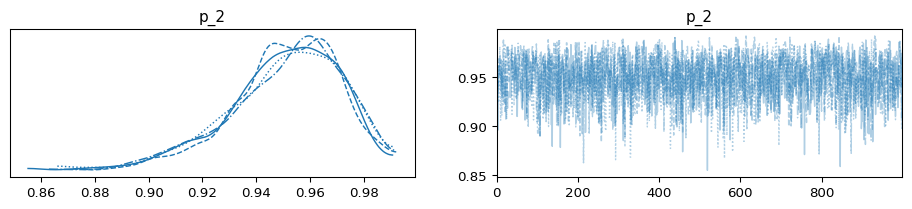
az.plot_trace(trace_2);
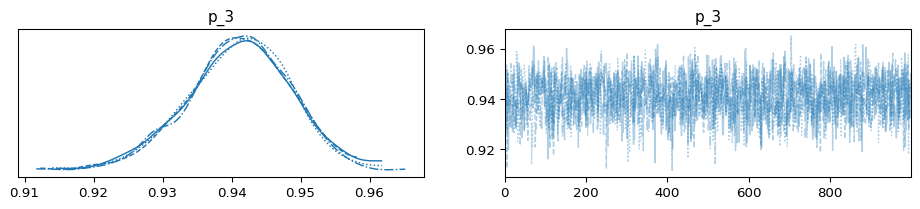
az.plot_trace(trace_3);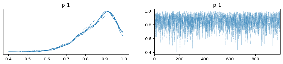

p1_summary = az.summary(trace_1, hdi_prob = 0.89)
p2_summary = az.summary(trace_2, hdi_prob = 0.89)
p3_summary = az.summary(trace_3, hdi_prob = 0.89)
summary = pd.concat([p1_summary, p2_summary, p3_summary])
summary

	mean	sd	hdi_5.5%	hdi_94.5%	mcse_mean	mcse_sd	ess_bulk	ess_tail	r_hat
p_1	0.856	0.092	0.733	0.990	0.002	0.002	1544.0	1382.0	1.0
p_2	0.951	0.021	0.920	0.984	0.000	0.000	1860.0	2288.0	1.0
p_3	0.941	0.007	0.929	0.952	0.000	0.000	1737.0	2772.0	1.0

Based on the table above, we can observe that seller #1 has a lower mean and a wider credible interval compared to seller #2 and seller #3. Now that we have the posterior parameter distributions, we can calculate the probability that buying from seller #2 would result in a better experience than buying from seller #1.

p1_samples = trace_1.posterior['p_1'].values.flatten()
p2_samples = trace_2.posterior['p_2'].values.flatten()
prob_s2_better = np.mean(p2_samples > p1_samples) * 100
print(f"Probability that seller 2 is better than seller 1: {prob_s2_better:.2f}%")

Probability that seller 2 is better than seller 1: 85.40%

Therefore, there is a good chance that you would have a better experience buying from seller #2 rather than seller #1.

Conclusion

In conclusion, with a relatively small amount of data, we face significant uncertainty regarding the true positive rate. Consequently, relying solely on the average of positive reviews can be misleading. However, with a substantial number of reviews, using the average of positive reviews becomes a reasonably sufficient metric.

Expand for Session Info

Click to view session information

-----
arviz               0.21.0
numpy               2.2.5
pandas              2.2.3
pymc                5.22.0
pytensor            2.30.3
session_info        v1.0.1
-----

Click to view modules imported as dependencies

PIL                         11.2.1
appnope                     0.1.4
arrow                       1.3.0
attr                        25.3.0
attrs                       25.3.0
babel                       2.17.0
cachetools                  5.5.2
certifi                     2025.04.26
charset_normalizer          3.4.1
cloudpickle                 3.1.1
comm                        0.2.2
cons                        0.4.6
cycler                      0.12.1
dateutil                    2.9.0.post0
debugpy                     1.8.14
decorator                   5.2.1
defusedxml                  0.7.1
distutils                   3.13.0
etuples                     0.3.9
executing                   2.2.0
filelock                    3.18.0
idna                        3.10
ipykernel                   6.29.5
jedi                        0.19.2
jinja2                      3.1.6
json5                       0.12.0
jsonpointer                 3.0.0
jsonschema                  4.23.0
jupyter_events              0.12.0
jupyter_server              2.15.0
jupyterlab_server           2.27.3
kiwisolver                  1.4.8
markupsafe                  3.0.2
matplotlib                  3.10.1
matplotlib_inline           0.1.7
more_itertools              10.3.0
multipledispatch            0.6.0
nbformat                    5.10.4
packaging                   25.0
parso                       0.8.4
platformdirs                4.3.7
prompt_toolkit              3.0.51
psutil                      7.0.0
pure_eval                   0.2.3
pydevd                      3.2.3
pygments                    2.19.1
pyparsing                   3.2.3
pytz                        2025.2
requests                    2.32.3
rfc3339_validator           0.1.4
rfc3986_validator           0.1.1
scipy                       1.15.2
setuptools                  80.1.0
six                         1.17.0
sniffio                     1.3.1
stack_data                  0.6.3
threadpoolctl               3.6.0
tornado                     6.4.2
traitlets                   5.14.3
unification                 0.4.6
urllib3                     2.4.0
wcwidth                     0.2.13
websocket                   1.8.0
xarray                      2025.4.0
xarray_einstats             0.8.0
yaml                        6.0.2
zmq                         26.4.0

-----
IPython             9.2.0
jupyter_client      8.6.3
jupyter_core        5.7.2
jupyterlab          4.4.1
notebook            7.4.1
-----
Python 3.13.0 (main, Oct  7 2024, 05:02:14) [Clang 15.0.0 (clang-1500.3.9.4)]
macOS-15.4.1-x86_64-i386-64bit-Mach-O
-----
Session information updated at 2025-05-01 09:44

Acknowledgments

This blogpost is heavily inspired by 3Blue1Brown video on Binomial distributions | Probabilities of probabilities.